This vignette describes the core functionality of the package by
identifying common trends in the longitudinal dataset that is included
with the package. We begin by loading the required package and the
latrendData dataset.
Initial data exploration
The latrendData is a synthetic dataset for which the
reference group of each trajectory is available, as indicated by the
Class column. We will use this column at the end of this
vignette to validate the identified model.
data(latrendData)
head(latrendData)
#>   Id      Time           Y   Class
#> 1  1 0.0000000 -1.08049205 Class 1
#> 2  1 0.2222222 -0.68024151 Class 1
#> 3  1 0.4444444 -0.65148373 Class 1
#> 4  1 0.6666667 -0.39115398 Class 1
#> 5  1 0.8888889 -0.19407876 Class 1
#> 6  1 1.1111111 -0.02991783 Class 1
Many of the functions of the package require the specification of the
trajectory identifier variable (named Id) and the time
variable (named Time). For convenience, we specify these
variables as package options.
options(latrend.id = "Id", latrend.time = "Time")Prior to attempting to model the data, it is worthwhile to visually inspect it.
plotTrajectories(latrendData, response = "Y")
Visualizing the trajectories of the latrend dataset.
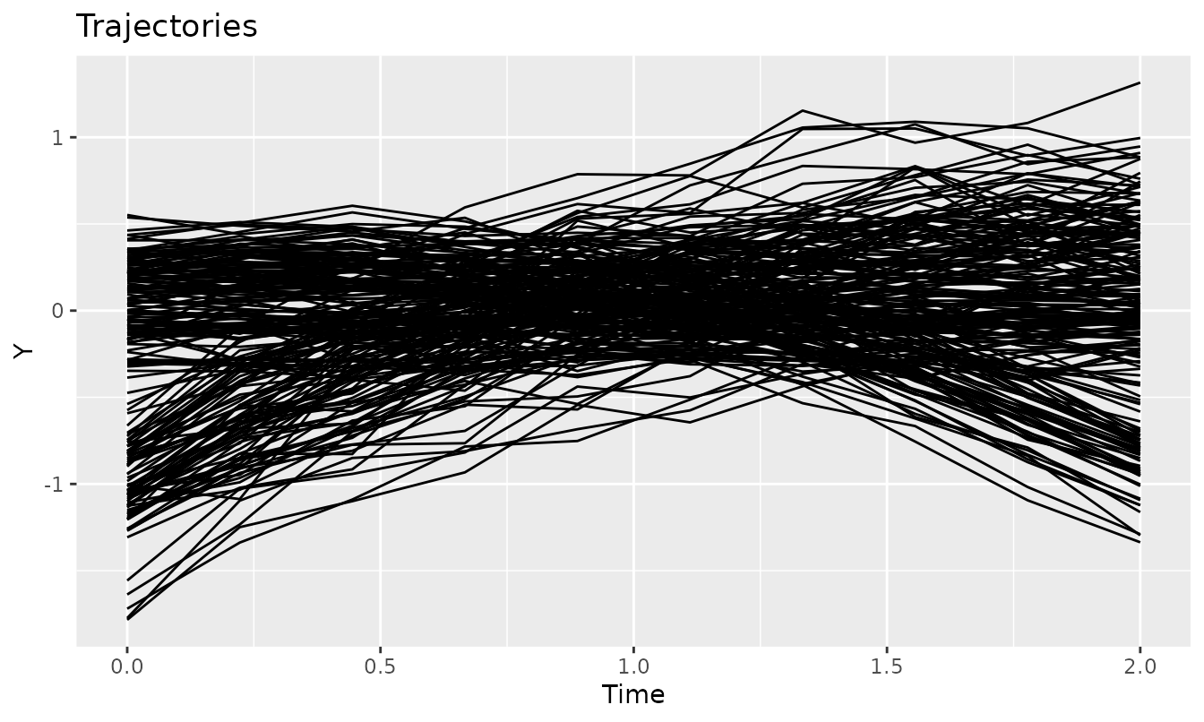
The presence of clusters is not apparent from the plot. With any longitudinal analysis, one should first consider whether clustering brings any benefit to the representation of heterogeneity of the data over a single common trend representation, or a multilevel model. In this demonstration, we omit this step under the prior knowledge that the data was generated via distinct mechanisms.
Non-parametric trajectory clustering
Assuming the appropriate (cluster) trajectory model is not known in advance, non-parametric longitudinal cluster models can provide a suitable starting point.
As an example, we apply longitudinal
k-means
(KML). First, we need to define the method. At the very least we need to
indicate the response variable the method should operate on. Secondly,
we should indicate how many clusters we expect. We do not need to define
the id and time arguments as we have set these
as package options. We use the nbRedrawing argument
provided by the KML package for reducing the number of repeated random
starts to only a single model estimation, in order to reduce the
run-time of this example.
kmlMethod <- lcMethodKML(response = "Y", nClusters = 2, nbRedrawing = 1)

kmlMethod
#> lcMethodKML specifying "longitudinal k-means (KML)"
#>  time:           getOption("latrend.time")
#>  id:             getOption("latrend.id")
#>  nClusters:      2
#>  nbRedrawing:    1
#>  maxIt:          200
#>  imputationMethod:"copyMean"
#>  distanceName:   "euclidean"
#>  power:          2
#>  distance:       function() {}
#>  centerMethod:   meanNA
#>  startingCond:   "nearlyAll"
#>  nbCriterion:    1000
#>  scale:          TRUE
#>  response:       "Y"
As seen in the output from the lcMethodKML object, the
KML method is defined by additional arguments. These are specific to the
kml package.
The KML model is estimated on the dataset via the
latrend function.
kmlModel <- latrend(kmlMethod, data = latrendData)
#>  ~ Fast KmL ~
#> *S
Now that we have fitted the KML model with 2 clusters, we can print a summary by calling:
kmlModel
#> Longitudinal cluster model using longitudinal k-means (KML)
#> lcMethodKML specifying "longitudinal k-means (KML)"
#>  time:           "Time"
#>  id:             "Id"
#>  nClusters:      2
#>  nbRedrawing:    1
#>  maxIt:          200
#>  imputationMethod:"copyMean"
#>  distanceName:   "euclidean"
#>  power:          2
#>  distance:       function () {}
#>  centerMethod:   `meanNA`
#>  startingCond:   "nearlyAll"
#>  nbCriterion:    1000
#>  scale:          TRUE
#>  response:       "Y"
#>
#> Cluster sizes (K=2):
#>         A         B
#> 120 (60%)  80 (40%)
#>
#> Number of obs: 2000, strata (Id): 200
#>
#> Scaled residuals:
#>     Min.  1st Qu.   Median     Mean  3rd Qu.     Max.
#> -3.57615 -0.62971  0.05638  0.00000  0.65400  3.20251
#> Attribution notice: lcModelKML makes use of external R package(s):
#>   - Run `getCitation(model)` to view how to cite the external package(s) when reporting results.
#>   - To disable this notice, set `options(latrend.cited.lcModelKML = TRUE)`.
Identifying the number of clusters
As we do not know the best number of clusters needed to represent the data, we should consider fitting the KML model for a range of clusters. We can then select the best representation by comparing the solutions by one or more cluster metrics.
We can specify a range of lcMethodKML methods based on a
prototype method using the lcMethods function. This method
outputs a list of lcMethod objects. A structured summary is
obtained by calling as.data.frame.
kmlMethods <- lcMethods(kmlMethod, nClusters = 1:7)

as.data.frame(kmlMethods)
#>        .class time id nClusters nbRedrawing maxIt imputationMethod distanceName
#> 1 lcMethodKML Time Id         1           1   200         copyMean    euclidean
#> 2 lcMethodKML Time Id         2           1   200         copyMean    euclidean
#> 3 lcMethodKML Time Id         3           1   200         copyMean    euclidean
#> 4 lcMethodKML Time Id         4           1   200         copyMean    euclidean
#> 5 lcMethodKML Time Id         5           1   200         copyMean    euclidean
#> 6 lcMethodKML Time Id         6           1   200         copyMean    euclidean
#> 7 lcMethodKML Time Id         7           1   200         copyMean    euclidean
#>   power      distance centerMethod startingCond nbCriterion scale response
#> 1     2 function() {}       meanNA    nearlyAll        1000  TRUE        Y
#> 2     2 function() {}       meanNA    nearlyAll        1000  TRUE        Y
#> 3     2 function() {}       meanNA    nearlyAll        1000  TRUE        Y
#> 4     2 function() {}       meanNA    nearlyAll        1000  TRUE        Y
#> 5     2 function() {}       meanNA    nearlyAll        1000  TRUE        Y
#> 6     2 function() {}       meanNA    nearlyAll        1000  TRUE        Y
#> 7     2 function() {}       meanNA    nearlyAll        1000  TRUE        Y
The list of lcMethod objects can be fitted using the
latrendBatch function, returning a list of
lcModel objects.
kmlModels <- latrendBatch(kmlMethods, data = latrendData, verbose = FALSE)

kmlModels
#> List of 7 lcModels with
#>   .name .method       seed nClusters
#> 1     1     kml 1753232290         1
#> 2     2     kml 1711075799         2
#> 3     3     kml  690659598         3
#> 4     4     kml  265368763         4
#> 5     5     kml  758296545         5
#> 6     6     kml 1649722645         6
#> 7     7     kml 2137634742         7
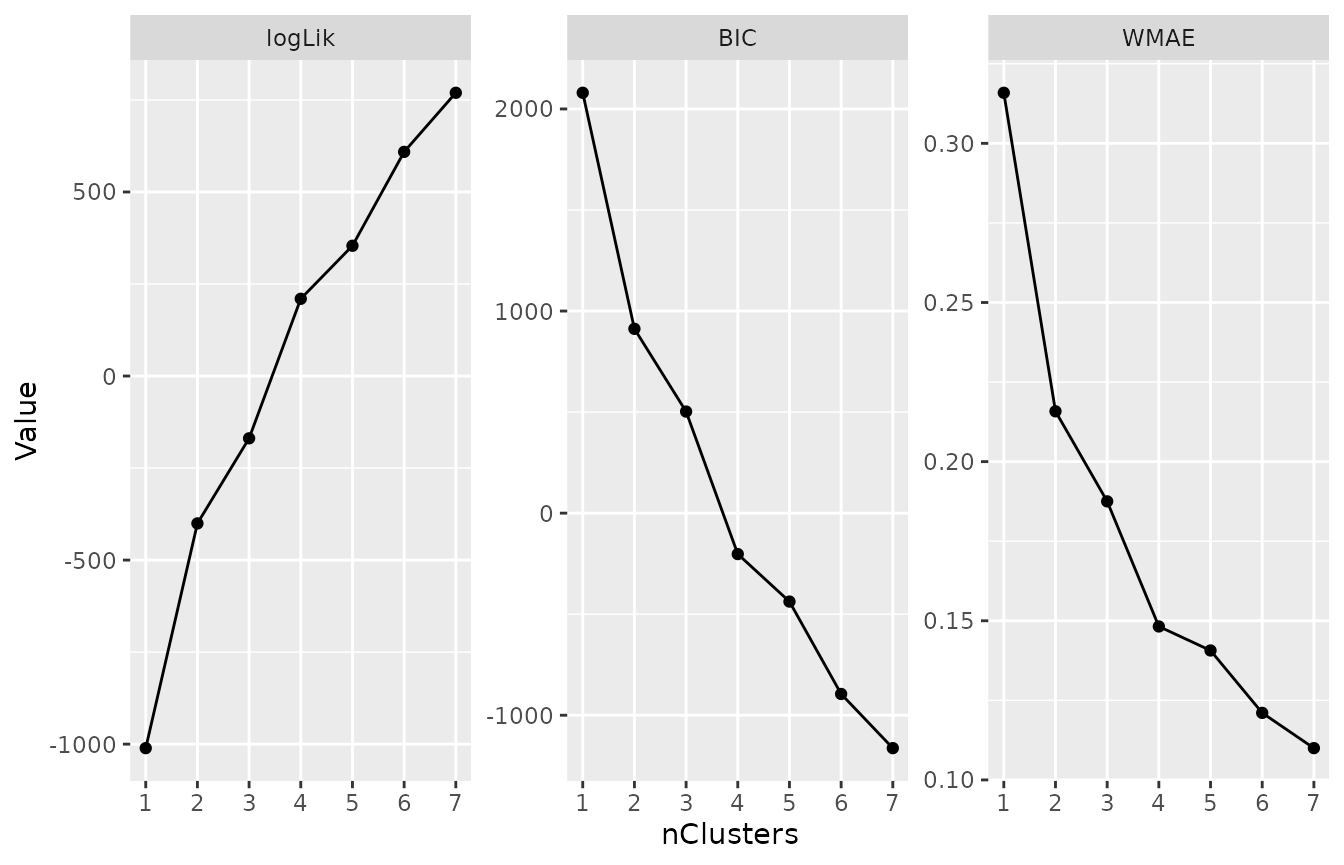
We can compare each of the solutions via one or more cluster metrics.
Considering the consistent improvements achieved by KML for an
increasing number of clusters, identifying the best solution by
minimizing a metric would lead to an overestimation. Instead, we perform
the selection via a manual elbow method, using the
plotMetric function.
plotMetric(kmlModels, c("logLik", "BIC", "WMAE"))Elbow plots of three relevant cluster metrics across the fitted models.
Investigating the preferred model
We have selected the 4-cluster model as the preferred representation.
We will now inspect this solution in more detail. Before we can start,
we first obtain the fitted lcModel object from the list of
fitted models.
kmlModel4 <- subset(kmlModels, nClusters == 4, drop = TRUE)

kmlModel4
#> Longitudinal cluster model using longitudinal k-means (KML)
#> lcMethodKML specifying "longitudinal k-means (KML)"
#>  seed:           265368763
#>  time:           "Time"
#>  id:             "Id"
#>  nClusters:      4
#>  nbRedrawing:    1
#>  maxIt:          200
#>  imputationMethod:"copyMean"
#>  distanceName:   "euclidean"
#>  power:          2
#>  distance:       function () {}
#>  centerMethod:   `meanNA`
#>  startingCond:   "nearlyAll"
#>  nbCriterion:    1000
#>  scale:          TRUE
#>  response:       "Y"
#>
#> Cluster sizes (K=4):
#>          A          B          C          D
#>   70 (35%)   50 (25%) 45 (22.5%) 35 (17.5%)
#>
#> Number of obs: 2000, strata (Id): 200
#>
#> Scaled residuals:
#>     Min.  1st Qu.   Median     Mean  3rd Qu.     Max.
#> -3.22269 -0.61623 -0.05837  0.00000  0.62240  3.63398
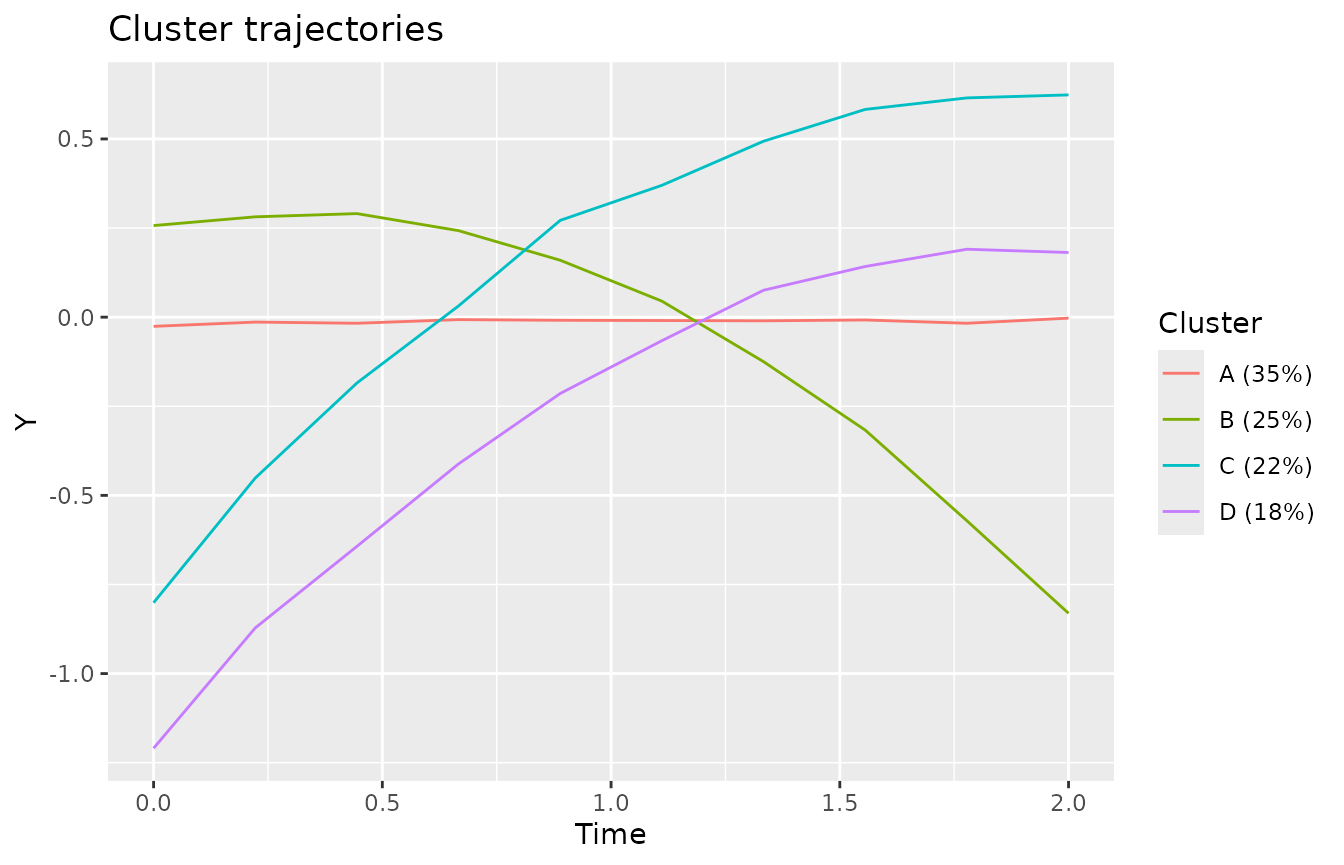
The plotClusterTrajectories function shows the estimated
cluster trajectories of the model.
plotClusterTrajectories(kmlModel4)Cluster trajectories for KML model with 4 clusters.
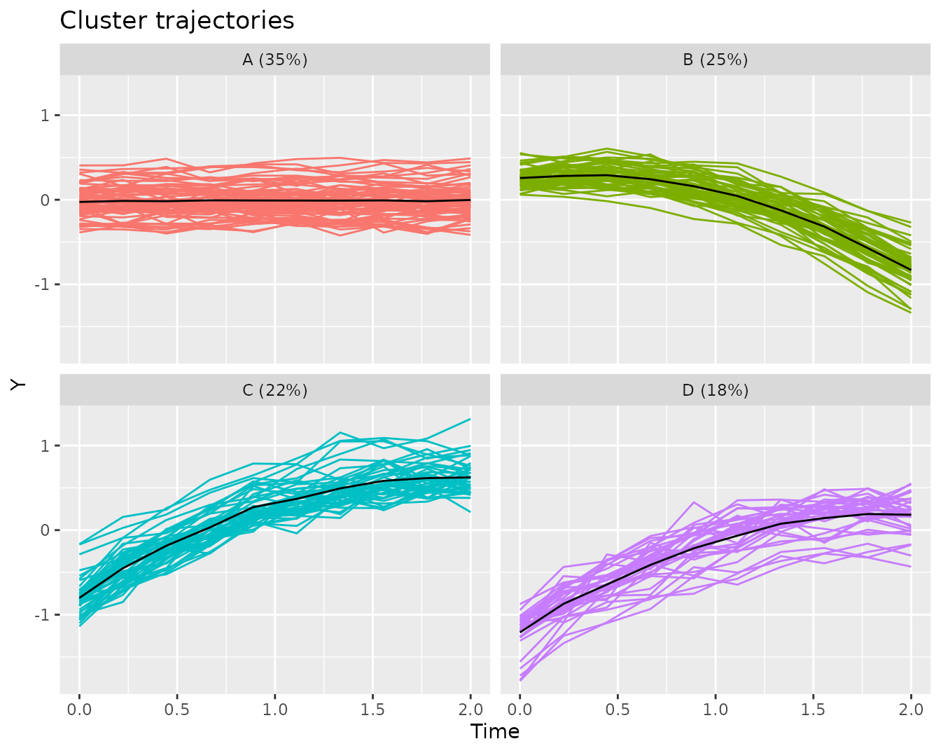
We can get a better sense of the representation of the cluster trajectories when plotted against the trajectories that have been assigned to the respective cluster.
plot(kmlModel4)Cluster trajectories for KML model with 4 clusters, along with the assigned trajectories.
The cluster assignment for each available subject is obtained using:
trajectoryAssignments(kmlModel4)
#>   [1] D C D C D D C C C D C C D D C C D C C C C C C D C C D D D C C D C C D D D
#>  [38] D C C D D C C D D C C D C C D C D C C D D C D C D C C D C D C C C C D C D
#>  [75] D C D C C D A A A A A A A A A A A A A A A A A A A A A A A A A A A A A A A
#> [112] A A A A A A A A A A A A A A A A A A A A A A A A A A A A A A A A A A A A A
#> [149] A A B B B B B B B B B B B B B B B B B B B B B B B B B B B B B B B B B B B
#> [186] B B B B B B B B B B B B B B B
#> Levels: A B C D
We can use this to construct a table of the cluster per subject, and merge it into the original data for further analysis.
# make sure to change the Id column name for your respective id column name
subjectClusters = data.frame(Id = ids(kmlModel4), Cluster = trajectoryAssignments(kmlModel4))
head(subjectClusters)
#>   Id Cluster
#> 1  1       D
#> 2  2       C
#> 3  3       D
#> 4  4       C
#> 5  5       D
#> 6  6       D

posthocAnalysisData = merge(latrendData, subjectClusters, by = 'Id')
head(posthocAnalysisData)
#>   Id      Time           Y   Class Cluster
#> 1  1 0.0000000 -1.08049205 Class 1       D
#> 2  1 0.2222222 -0.68024151 Class 1       D
#> 3  1 0.4444444 -0.65148373 Class 1       D
#> 4  1 0.6666667 -0.39115398 Class 1       D
#> 5  1 0.8888889 -0.19407876 Class 1       D
#> 6  1 1.1111111 -0.02991783 Class 1       D
aggregate(Y ~ Cluster, posthocAnalysisData, mean)
#>   Cluster           Y
#> 1       A -0.01200153
#> 2       B -0.05675290
#> 3       C  0.15509611
#> 4       D -0.28265770
Model adequacy
The list of currently supported internal model metrics can be
obtained by calling the getInternalMetricNames
function.
getInternalMetricNames()
#>  [1] "AIC"              "APPA.mean"        "APPA.min"         "ASW"
#>  [5] "BIC"              "CAIC"             "CalinskiHarabasz" "CLC"
#>  [9] "converged"        "DaviesBouldin"    "deviance"         "Dunn"
#> [13] "ED"               "ED.fit"           "entropy"          "estimationTime"
#> [17] "ICL.BIC"          "logLik"           "MAE"              "Mahalanobis"
#> [21] "MSE"              "RE"               "relativeEntropy"  "RMSE"
#> [25] "RSS"              "scaledEntropy"    "SED"              "SED.fit"
#> [29] "sigma"            "ssBIC"            "WMAE"             "WMSE"
#> [33] "WRMSE"            "WRSS"
As an example, we will compute the APPA (a measure of cluster separation), and the WRSS and WMAE metrics (measures of model error).
metric(kmlModel, c("APPA.mean", "WRSS", "WMAE"))
#>   APPA.mean        WRSS        WMAE
#>   0.9999979 152.7557738   0.2158131
The quantile-quantile (QQ) plot can be used to assess the model for structural deviations.
qqPlot(kmlModel4)QQ-plot of the selected KML model.
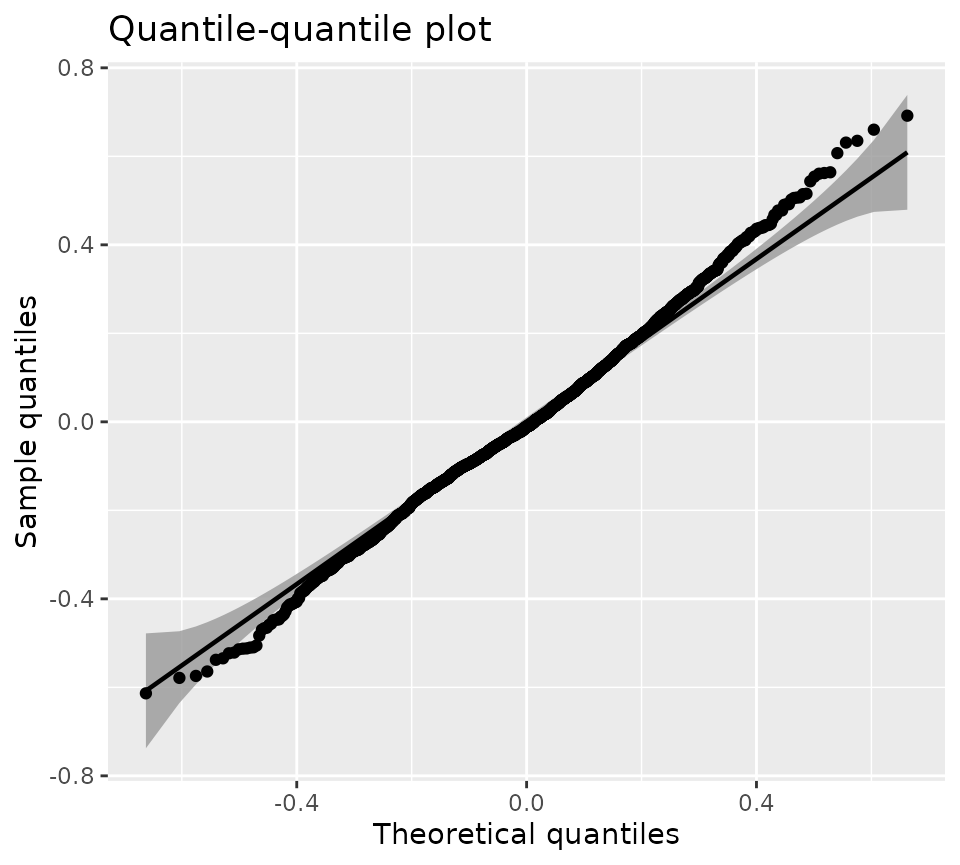
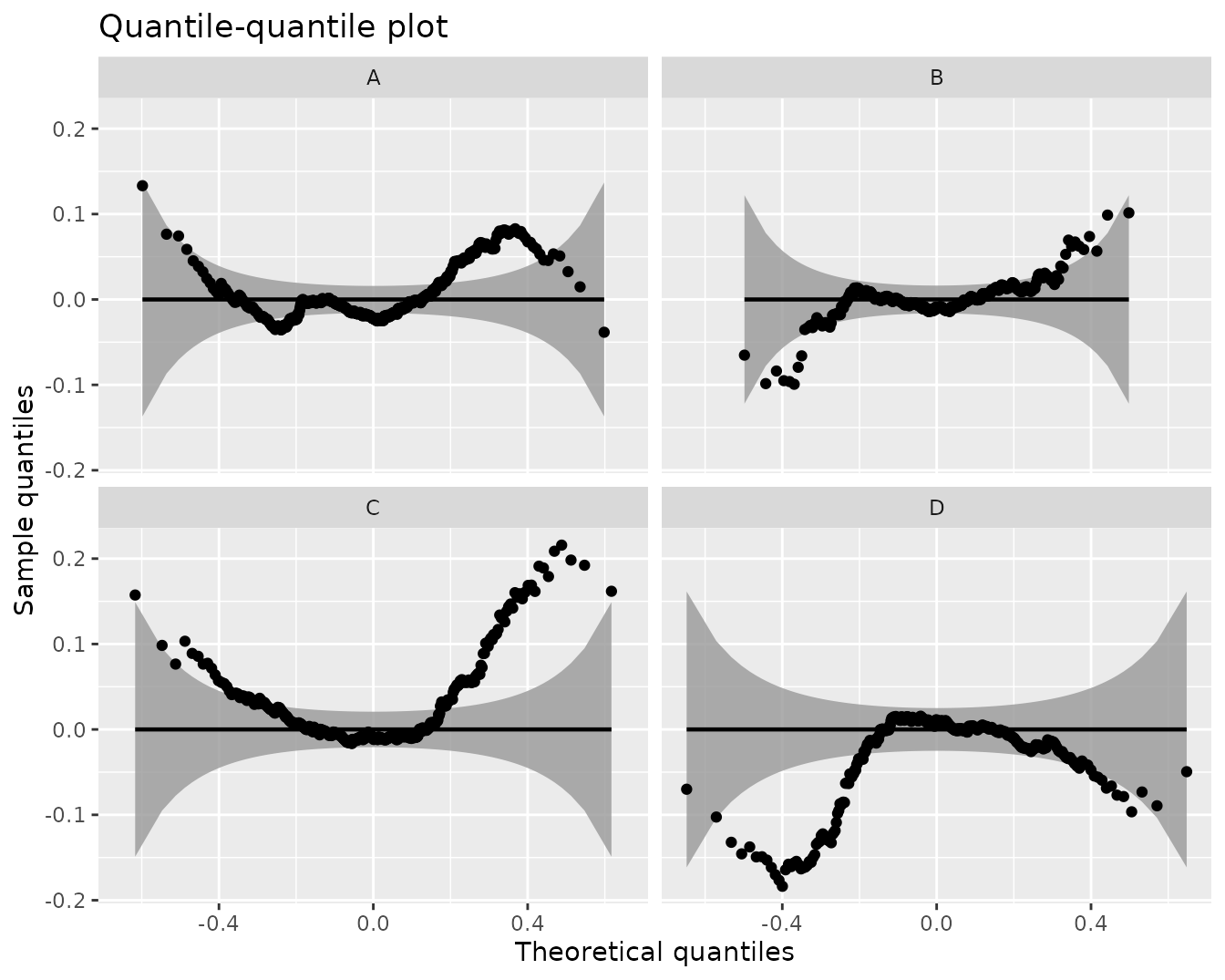
Overall, the unexplained errors closely follow a normal distribution. In situations where structural deviations from the expected distribution are apparent, it may be fruitful to investigate the QQ plot on a per-cluster basis.
qqPlot(kmlModel4, byCluster = TRUE, detrend = TRUE)Cluster-specific detrended QQ-plot for the selected KML model.
Parametric trajectory clustering
The KML analysis has provided us with clues on an appropriate model for the cluster trajectories. We can use these insights to define a parametric representation of each of the trajectories and cluster them using k-means.
lmkmMethod <- lcMethodLMKM(formula = Y ~ Time)

lmkmMethod
#> lcMethodLMKM specifying "lm-kmeans"
#>  time:           getOption("latrend.time")
#>  id:             getOption("latrend.id")
#>  nClusters:      2
#>  center:         meanNA
#>  standardize:    scale
#>  method:         "qr"
#>  model:          TRUE
#>  y:              FALSE
#>  qr:             TRUE
#>  singular.ok:    TRUE
#>  contrasts:      NULL
#>  iter.max:       10
#>  nstart:         1
#>  algorithm:      c("Hartigan-Wong", "Lloyd", "Forgy", "Ma
#>  formula:        Y ~ Time
We fit LMKM for 1 to 4 clusters.
lmkmMethods <- lcMethods(lmkmMethod, nClusters = 1:5)

lmkmModels <- latrendBatch(lmkmMethods, data = latrendData, verbose = FALSE)plotMetric(lmkmModels, c("logLik", "BIC", "WMAE"))Three cluster metrics for each of the GBTMs.
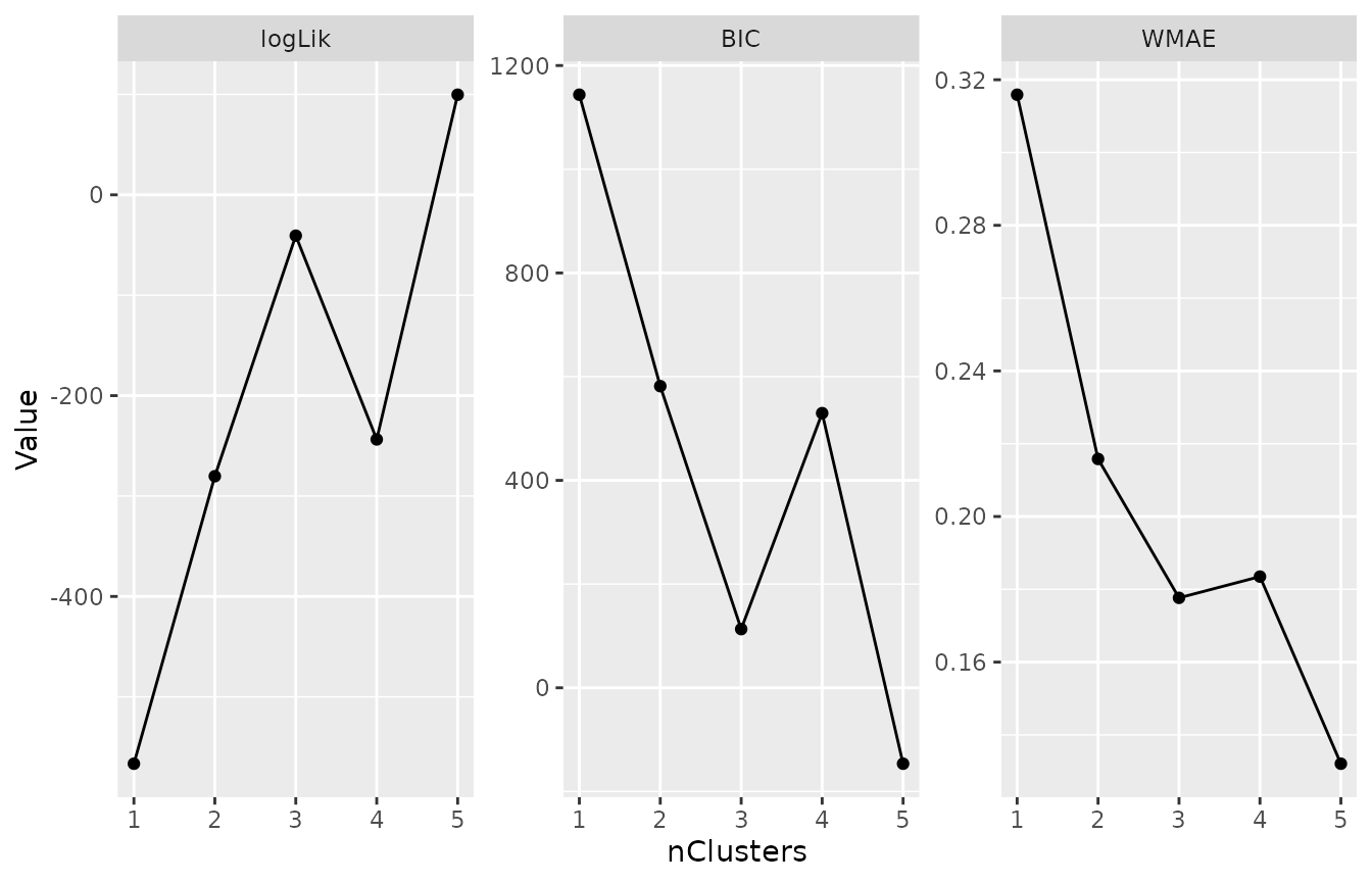
All metrics clearly point to the three-cluster solution.
Comparison to the reference
Since we have established a preferred clustered representation of the
data heterogeneity, we can now compare the resulting cluster assignments
to the ground truth from which the latrendData data was
generated.
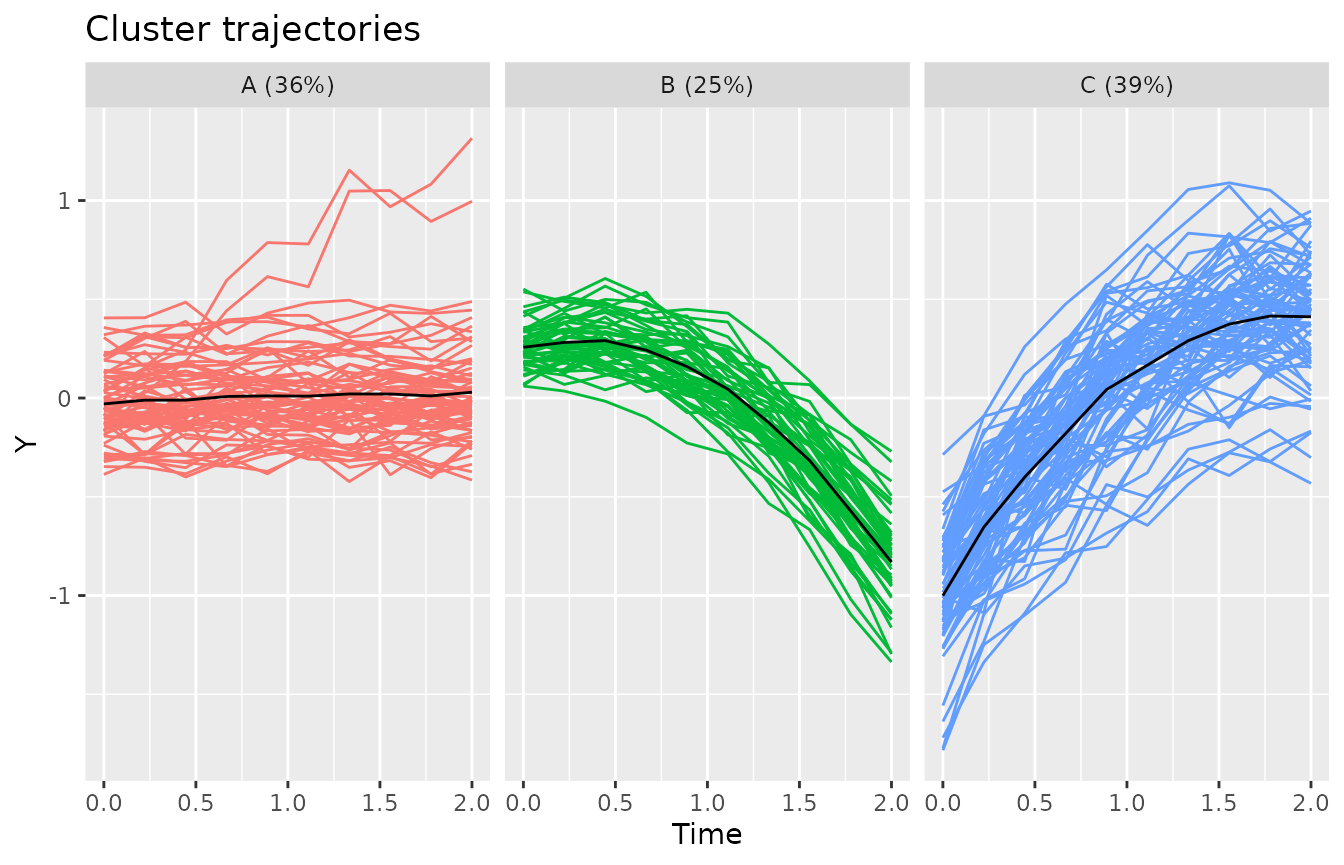
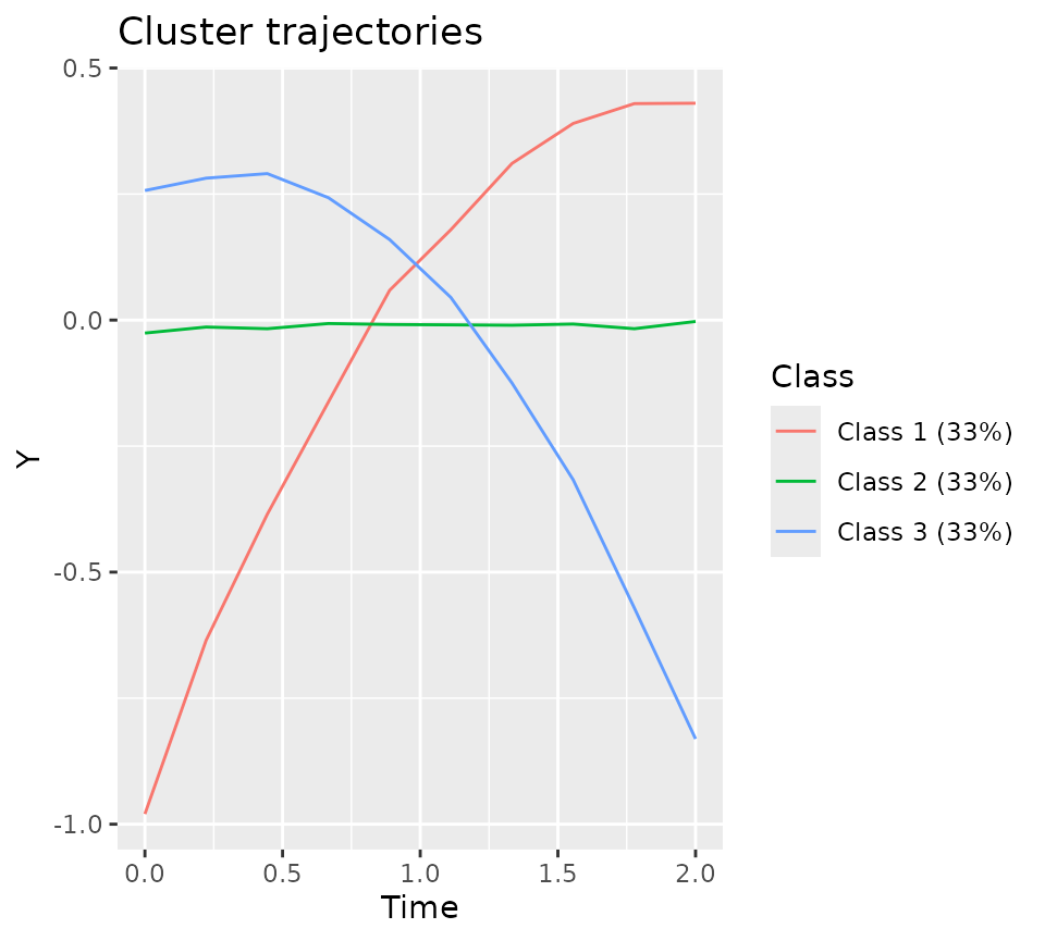
Using the reference assignments, we can also plot a non-parametric estimate of the cluster trajectories. Note how it looks similar to the cluster trajectories found by our model.
plotClusterTrajectories(latrendData, response = "Y", cluster = "Class")Non-parametric estimates of the cluster trajectories based on the reference assignments.
In order to compare the reference assignments to the trajectory
assignments generated by our model, we can create a lcModel
object based on the reference assignments using the
lcModelPartition function.
refTrajAssigns <- aggregate(Class ~ Id, data = latrendData, FUN = data.table::first)
refModel <- lcModelPartition(data = latrendData, response = "Y", trajectoryAssignments = refTrajAssigns$Class)
refModel
#> Longitudinal cluster model using part
#> lcMethod specifying "undefined"
#> no arguments
#>
#> Cluster sizes (K=3):
#>  Class 1  Class 2  Class 3
#> 80 (40%) 70 (35%) 50 (25%)
#>
#> Number of obs: 2000, strata (Id): 200
#>
#> Scaled residuals:
#>     Min.  1st Qu.   Median     Mean  3rd Qu.     Max.
#> -3.67125 -0.55452 -0.04079 0.00000 0.58663 3.76931plot(refModel)Cluster trajectories of the reference model.
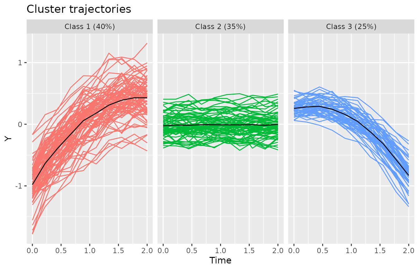
By constructing a reference model, we can make use of the
standardized way in which lcModel objects can be compared.
A list of supported comparison metrics can be obtained via the
getExternalMetricNames function.
getExternalMetricNames()
#>  [1] "adjustedRand"   "CohensKappa"    "F"              "F1"
#>  [5] "FolkesMallows"  "Hubert"         "Jaccard"        "jointEntropy"
#>  [9] "Kulczynski"     "MaximumMatch"   "McNemar"        "MeilaHeckerman"
#> [13] "MI"             "Mirkin"         "NMI"            "NSJ"
#> [17] "NVI"            "Overlap"        "PD"             "Phi"
#> [21] "precision"      "Rand"           "recall"         "RogersTanimoto"
#> [25] "RusselRao"      "SMC"            "SokalSneath1"   "SokalSneath2"
#> [29] "splitJoin"      "splitJoin.ref"  "VI"             "Wallace1"
#> [33] "Wallace2"       "WMMAE"          "WMMAE.ref"      "WMMSE"
#> [37] "WMMSE.ref"      "WMRSS"          "WMRSS.ref"
Lastly, we compare the agreement in trajectory assignments via the adjusted Rand index.
externalMetric(bestLmkmModel, refModel, "adjustedRand")
#> adjustedRand
#>    0.9669189
With a score of
externalMetric(bestLmkmModel, refModel, "adjustedRand"), we
have a near-perfect match. This result is expected, as the dataset was
generated using a growth mixture model.