In this vignette we demonstrate how to define new methods.
Case study data
We will generate a dataset comprising two clusters with a different intercept and slope. Firstly, we configure the default id, time, and response variable, so that these do not need to be provided to the other function calls.
library(latrend)
library(data.table)
options(
  latrend.id = "Traj",
  latrend.time = "Time",
  latrend.verbose = TRUE
)
Next, we generate the dataset, with 40 trajectories for cluster A and 60 trajectories for cluster B. Cluster A involves trajectories with a downward slope, whereas cluster B has an upward slope. We define a fixed mean of 1, such that all the cluster trajectories are shifted, placing cluster A at intercept 2, and cluster B at intercept 1.
set.seed(1)
casedata <- generateLongData(
  sizes = c(40, 60),
  data = data.frame(Time = 0:10),
  fixed = Y ~ 1,
  fixedCoefs = 1,
  cluster = ~ Time,
  clusterCoefs = cbind(c(2, -.1), c(0, .05)),
  random = ~ Time,
  randomScales = cbind(c(.2, .02), c(.2, .02)),
  noiseScales = .05
) %>%
  as.data.table()
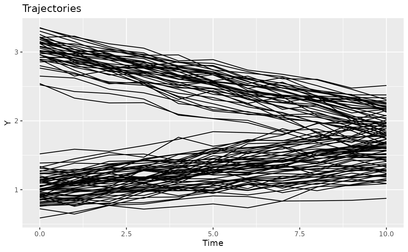
We plot the data to get a sense of different trajectories that have been generated. Visually, there is little group separation.
plotTrajectories(casedata, response = "Y")
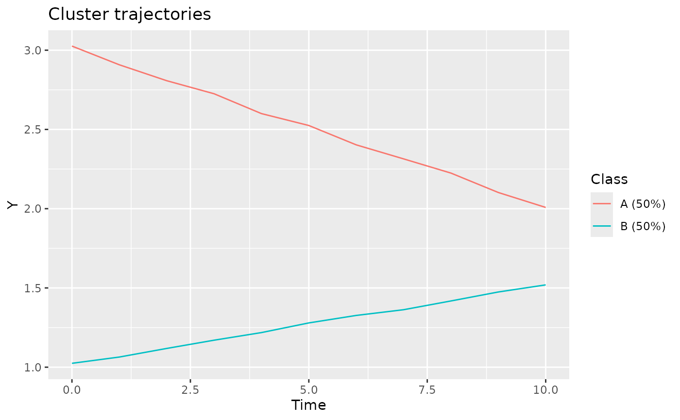
Since we generated the data, we have the luxury of looking at
reference cluster trajectories, as stored in the Mu.cluster
column. Note that Mu.fixed must be added to obtain the
correct values.
plotClusterTrajectories(casedata, response = "Y", cluster = "Class")
Stratification
Rather than starting with clustering, in some case studies there may be prior knowledge on how to sensibly stratify the trajectories. Either by an observed independent variable (e.g., age or gender), or a certain aspect of the observed trajectory (e.g., the intercept, slope, variability).
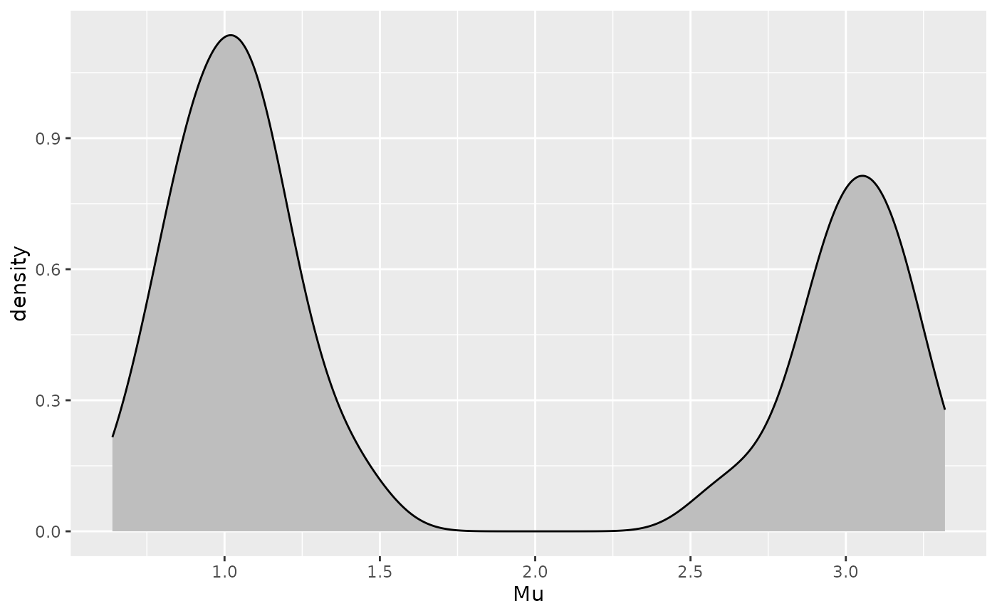
Let’s presume in this example that domain knowledge suggests that stratifying by the intercept may provide a sensible grouping of the trajectories. This approach is further supported by the density plot of the trajectory intercepts, which shows a bimodal distribution.
ggplot(casedata[Time == 0], aes(x = Mu)) +
  geom_density(fill = "gray", adjust = .3)
Based on the density plot, we will assign trajectories with an intercept above 1.6 to cluster A, and the remainder to cluster B.
method <- lcMethodStratify(response = "Y", Y[1] > 1.6)
model <- latrend(method, casedata)clusterProportions(model)
#> A B
#> 0.6 0.4The approach we specified requires the first observation to be available, and is sensitive to noise. A more robust alternative would be to fit a linear model per trajectory, and to use the estimated intercept to stratify the trajectories on.
We can specify this stratification model by defining a function which takes the data of separate trajectories as input. This function should return a single cluster assignment for the respective trajectory. By returning a factor, we can pre-specify the cluster names.
stratfun <- function(data) {
  int <- coef(lm(Y ~ Time, data))[1]
  factor(int > 1.7, levels = c(FALSE, TRUE), labels = c("Low", "High"))
}
m2 <- lcMethodStratify(response = "Y", stratify = stratfun, center = mean)
model2 <- latrend(m2, casedata)

clusterProportions(model2)
#>  Low High
#>  0.6  0.4
In case the linear regression step is time-intensive, a more efficient approach is to save the pre-computed trajectory intercepts as a column in the original data. This column can then be referred to in the expression of the stratification model.
casedata[, Intercept := coef(lm(Y ~ Time, .SD))[1], by = Traj]

m3 <- lcMethodStratify(
  response = "Y",
  stratify = Intercept[1] > 1.7,
  clusterNames = c("Low", "High")
)
model3 <- latrend(m3, casedata)
Two-step clustering
We can take the approach involving the estimation of a linear model per trajectory one step further. Instead of using a pre-defined threshold on the intercept, we use a cluster algorithm on both the intercept and slope to automatically find clusters.
We first define the representation step, which estimates the model
coefficients per trajectory, and outputs a matrix with the
coefficients per trajectory per row.
repStep <- function(method, data, verbose) {
  dt <- as.data.table(data)
  coefdata <- dt[, lm(Y ~ Time, .SD) %>% coef() %>% as.list(), keyby = Traj]
  coefmat <- subset(coefdata, select = -1) %>% as.matrix()
  rownames(coefmat) <- coefdata$Traj
  coefmat
}
The cluster step takes the coefficient matrix as input. A
cross-sectional cluster algorithm can then be applied to the matrix. In
this example, we apply
k-means.
The cluster step should output a lcModel object.
The lcModelPartition function creates a
lcModel object for a given vector of cluster
assignments.
clusStep <- function(method, data, repMat, envir, verbose) {
  km <- kmeans(repMat, centers = 3)

  lcModelPartition(
    response = method$response,
    data = data,
    trajectoryAssignments = km$cluster,
    center = method$center,
    method = method,
    model = km
  )
}
We are now ready to create the lcMethodFeature
method.
m.twostep <- lcMethodFeature(
  response = "Y",
  representationStep = repStep,
  clusterStep = clusStep
)
model.twostep <- latrend(m.twostep, data = casedata)
summary(model.twostep)
#> Longitudinal cluster model using part
#> lcMethodFeature specifying "two-step clustering"
#> standardize: `scale`
#> center: `meanNA`
#> time: "Time"
#> id: "Traj"
#> response: "Y"
#> representationStep:`repStep`
#> clusterStep: `clusStep`
#>
#> Cluster sizes (K=3):
#> A B C
#> 35 (35%) 25 (25%) 40 (40%)
#>
#> Number of obs: 1100, strata (Traj): 100
#>
#> Scaled residuals:
#> Min. 1st Qu. Median Mean 3rd Qu. Max.
#> -3.08943 -0.67260 0.03618 0.00000 0.73723 2.64516General approach
The two-step model defined above is hard-coded for a given formula
and a fixed number of clusters. In an exploratory setting, it is
convenient to define a parameterized method. Here, we change the two
functions to take arguments through the lcMethod object in
the method variable.
Note that we can introduce new arguments which are not originally
part of lcMethodFeature (e.g., nClusters) to
enable the specification of the number of clusters in our method.
repStep.gen <- function(method, data, verbose) {
  dt <- as.data.table(data)
  coefdata <- dt[, lm(method$formula, .SD) %>% coef() %>% as.list(), keyby = c(method$id)]
  # exclude the id column
  coefmat <- subset(coefdata, select = -1) %>% as.matrix()
  rownames(coefmat) <- coefdata[[method$id]]
  coefmat
}

clusStep.gen <- function(method, data, repMat, envir, verbose) {
  km <- kmeans(repMat, centers = method$nClusters)

  lcModelPartition(
    response = method$response,
    data = data,
    trajectoryAssignments = km$cluster,
    center = method$center,
    method = method,
    model = km
  )
}
We create a new lcMethodFeature instance with the more
generic functions. Defining values for formula and
nClusters here makes these arguments values act as default
values in a call of latrend.
m.twostepgen <- lcMethodFeature(
  response = "Y",
  representationStep = repStep.gen,
  clusterStep = clusStep.gen
)
However, because we omitted the specification of formula
and nClusters, these need to be provided in the
latrend call.
model.twostepgen <- latrend(m.twostepgen, formula = Y ~ Time, nClusters = 2, casedata)
summary(model.twostepgen)
#> Longitudinal cluster model using part
#> lcMethodFeature specifying "two-step clustering"
#>  nClusters:      2
#>  formula:        Y ~ Time
#>  standardize:    `scale`
#>  center:         `meanNA`
#>  time:           "Time"
#>  id:             "Traj"
#>  response:       "Y"
#>  representationStep:`repStep.gen`
#>  clusterStep:    `clusStep.gen`
#>
#> Cluster sizes (K=2):
#>        A        B
#> 40 (40%) 60 (60%)
#>
#> Number of obs: 1100, strata (Traj): 100
#>
#> Scaled residuals:
#>    Min. 1st Qu.  Median    Mean 3rd Qu.    Max.
#> -2.9747 -0.6992  0.0589  0.0000  0.6958  2.9260